Basic Webscraping with Python
A Basic Introduction to Webscraping in Python
Webscraping generally refers to the process of extracting data or information from websites. As such, it offers a great way to unlock new data sources and is hence useful for researchers, academics, and professionals alike.
Webscraping comes in many different shapes and forms. Similarly, Python offers various packages and libraries that simplify webscraping and webautomation tasks, all of which have their unique set of strengths and weaknesses. To keep things simple, I will focus on a rather straightforward example in this tutorial.
1 HTML
HTML stands for Hyper Text Markup Language. Markup languages are designed to annotate or format text. Once the document is displayed, only the content is visible. This is similar to what we do when we set up a LaTeX document. We use general tagging conventions to define and format the document, which translate into stylistic features once the document is compiled. The annotations themselves are then invisible to the reader. The standard markup language used whenever content is to be displayed on a website is HTML. As with a LaTeX compiler, a webbrowser interprets the HTML annotations in the background and only displays the actual content of the document to the reader. The underlying code is what we see when we e.g. accidentally hit “inspect” while browsing on a website (more on this later). To gain an understanding of webscraping, a very basic introduction to HTML thus seems inevitable.
One important building block of HTML markup are so-called tags. A HTML document is composed of nested HTML elements. Different elements are indicated by different tags. Tags usually come in pairs, where the first tag defines the start and the second tag defines the end. For illustration purposes, the code below creates an example HTML document:
<!DOCTYPE html>
<html>
  <head>
    <title>This is a the browser page title</title>
  </head>
  <body>
    <div>
        <h3> This is a level 3 header </h3>
        <p> Here we have <br> some text </p>
    </div>
  </body>
</html>
When typing the above code e.g. into a Markdown cell in a Jupyter Notebook, we can see what the interpreted document looks like:
<!DOCTYPE html>
This is a level 3 header
Here we have
some text
As we can see, the markup indeed vanishes. The <h3> </h3> tag pair is e.g. interpreted as a level 3 header, while the text content is enclosed in the <p> </p> tag pair. The <br> does not have a “twin” and introduces a line break. Of course, real websites are way more complex and HTML comes with many more tag pairs and other bells and whistles. Nonetheless, the general principle holds.
2 Webscraping
2.0 A First Glance
To locate the content that we want to scrape on a website, we thus have to make our way through the “tree” and identify the relevant HTML tag that encloses the content of interest. When building a basic webscraping algorithm, this is actually the main task.
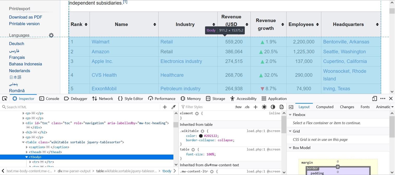
To make things a little more interesting, suppose we are interested in scraping the list of the largest 500 US companies by revenue from Wikipedia. Highlighting e.g. the first table entry, right-clicking and then selecting “inspect” opens the below view:
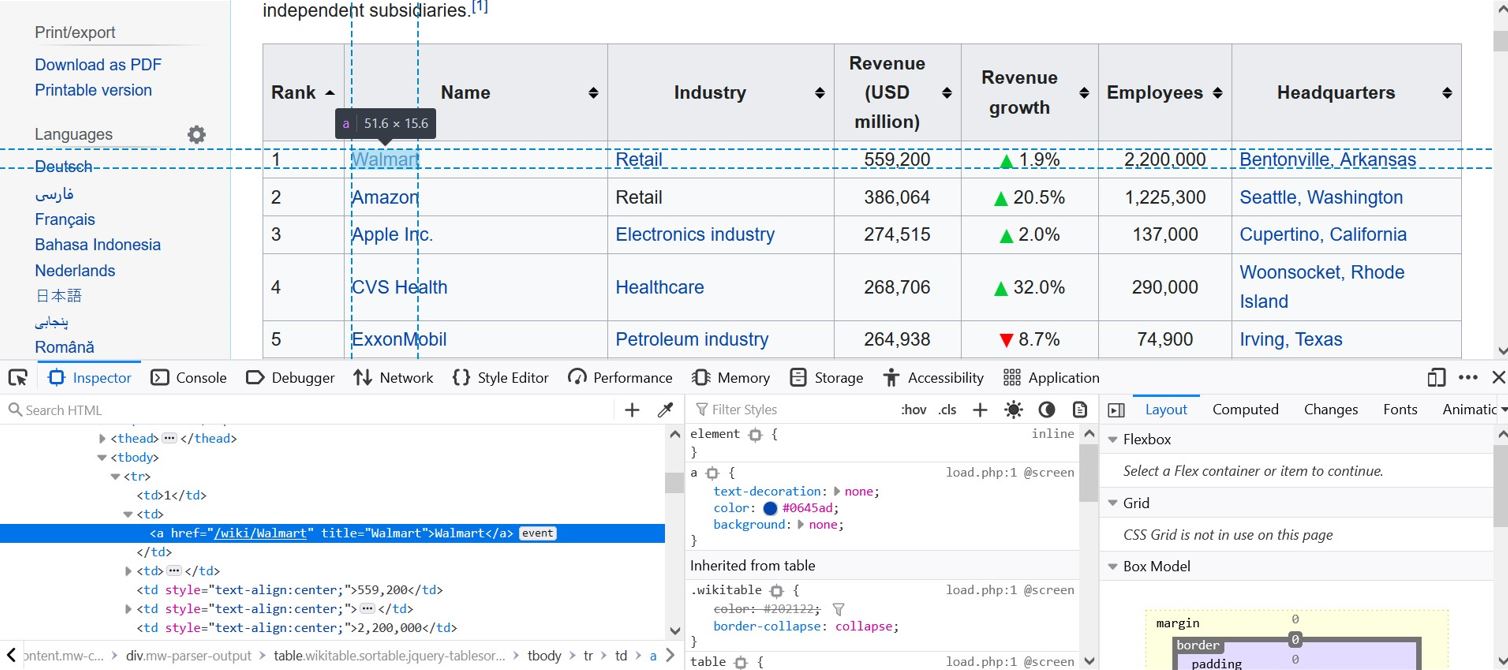
I am using Firefox here, but the same works with other browsers. As we can see, the table content is enclosed by the HTML tag pair <tbody> </tbody>. Hovering around with the mouse, we can see that the first table row is contained in the first <tr> </tr> tag pair. Within the first row, the different columns are enclosed in <td> </td> tag pairs. While columns with numerical values or plain text appear directly between the <td> </td> tags, links such as company names are enclosed in <a> </a> tags.
More specifically, the first table row looks like this:
<tbody>
<tr>
<td>1
</td>
<td><a href="/wiki/Walmart" title="Walmart">Walmart</a>
</td>
<td><a href="/wiki/Retail" title="Retail">Retail</a>
</td>
<td style="text-align:center;">559,200
</td>
<td style="text-align:center;"><img alt="Increase" src="//upload.wikimedia.org/wikipedia/commons/thumb/b/b0/Increase2.svg/11px-Increase2.svg.png" decoding="async" title="Increase" srcset="//upload.wikimedia.org/wikipedia/commons/thumb/b/b0/Increase2.svg/17px-Increase2.svg.png 1.5x, //upload.wikimedia.org/wikipedia/commons/thumb/b/b0/Increase2.svg/22px-Increase2.svg.png 2x" data-file-width="300" data-file-height="300" width="11" height="11"> <span data-sort-value="7000300000000000000" style="display:none"></span> 1.9%
</td>
<td style="text-align:center;">2,200,000
</td>
<td><a href="/wiki/Bentonville,_Arkansas" title="Bentonville, Arkansas">Bentonville, Arkansas</a>
</td>
</tr>
...
This is exactly the structure we seek to exploit with our webscraping algorithm when downloading the data.
2.1 Writing a Simple Webscraper
As I said before, we are going to focus on what is the simplest approach in my opinion. There exist many other elegant alternatives and I often find myself using different approaches for different use cases. Before we start, however, we need to import the necessary libraries
import requests       # HTTP library for requesting website
from lxml import html # library for processing HTML
from lxml import etree
With these two libraries on board, we can get started.
Making a HTTP request
As a first step, we simply plug the website’s URL into the requests.get() method. The resulting response object now contains all the necessary information.
response = requests.get(url="https://en.wikipedia.org/wiki/List_of_largest_companies_in_the_United_States_by_revenue")
print(response.status_code)
200
To access the content, we now use the lxml library:
# extract the content
tree = html.fromstring(response.content)

# display the first 1000 elements of the HTML document
print(etree.tostring(tree, pretty_print=True, method="html")[:1000])
b'<html class="client-nojs" lang="en" dir="ltr">\n<head>\n<meta charset="UTF-8">\n<title>List of largest companies in the United States by revenue - Wikipedia</title>\n<script>document.documentElement.className="client-js";RLCONF={"wgBreakFrames":!1,"wgSeparatorTransformTable":["",""],"wgDigitTransformTable":["",""],"wgDefaultDateFormat":"dmy","wgMonthNames":["","January","February","March","April","May","June","July","August","September","October","November","December"],"wgRequestId":"26ad4969-72d1-4b32-9322-b11074152b81","wgCSPNonce":!1,"wgCanonicalNamespace":"","wgCanonicalSpecialPageName":!1,"wgNamespaceNumber":0,"wgPageName":"List_of_largest_companies_in_the_United_States_by_revenue","wgTitle":"List of largest companies in the United States by revenue","wgCurRevisionId":1041408636,"wgRevisionId":1041408636,"wgArticleId":61181662,"wgIsArticle":!0,"wgIsRedirect":!1,"wgAction":"view","wgUserName":null,"wgUserGroups":["*"],"wgCategories":["Articles with short description","Short description'
Xpath
We could now navigate through the parse tree by hand, identify our elements of interest and simply read out the content. This not only sounds cumbersome, it also is! Luckily, there is a faster way.
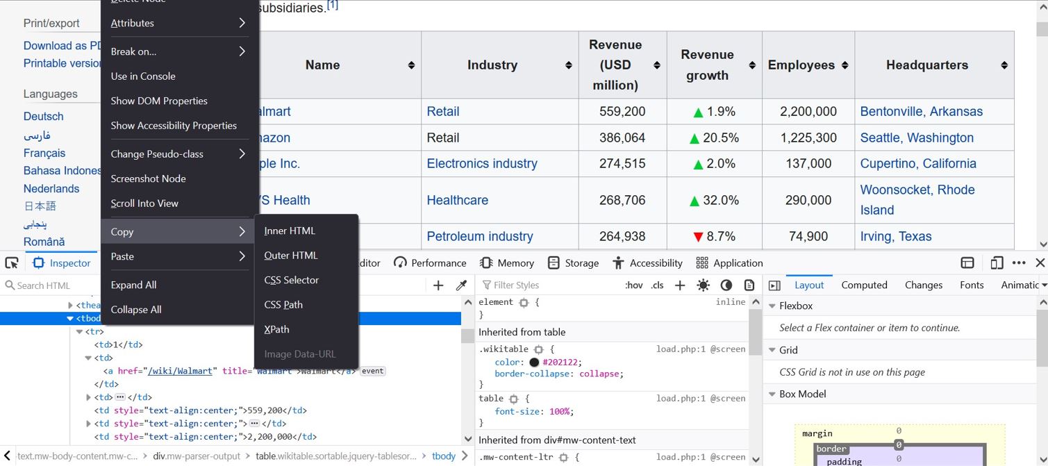
xpath is a so-called query language. With its help, we can easily jump directly to relevant branches in our tree. The neat thing is that the inspect tool in browsers like firefox, hands the relevant xpath directly to us. Simply right-clicking the tbody element, navigating to “copy” and selecting “xpath”, copies the xpath to the clip board.

We can now plug the xpath into the xpath method of our tree object:
table = tree.xpath('/html/body/div[3]/div[3]/div[5]/div[1]/table[2]/tbody')
table
[<Element tbody at 0x2122fa344f0>]
As we can see, table is a list containing the tbody element. All we need to do now is recall which tags enclose the rows and columns of our table. We can then simply read out the elements of interest.
# initialize an empty dictionary
dic = {}

# a loop iterating through the rows of the table starting in the second row
for row in table[0].findall('tr')[1:]:

    # find all <td> tags in row
    td = row.findall('td')

    # read out the company rank/text in the first coulumn
    rank = td[0].xpath("string()").strip()


    # read out the company name/text in the second coulumn
    name = td[1].xpath('string()').strip()

    # read out the company's industry/text in the third coulumn
    industry = td[2].xpath('string()').strip()

    # read out the company's revenue/text in the fourth coulumn
    revenue = td[3].xpath('string()').strip()

    # read out the company's revenue growth/text in the fifth coulumn
    revenue_growth = td[4].xpath('string()').strip()

    # read out the company's number of employees/text in the sixth coulumn
    employees = td[5].xpath('string()').strip()

    # read out the company's headquarter location/text in the last coulumn
    HQ = td[6].xpath('string()').strip()

    # save the information in a dictionary
    dic[name] = {'rank' : rank, 'industry' : industry, 'revenue' : revenue, 'revenue growth' : revenue_growth,
                 'employees': employees, 'HQ' : HQ}
To read out the individual text content, I again use xpath. The strip method sanitizes the
resulting string an removes e.g. \n tags. The same result can be achieved without using xpath and
using the text and text_content() methods instead. There is some subtle differences between
the methods, but they do not matter here.
# initialize an empty dictionary
dic = {}

# a loop iterating through the rows of the table starting in the second row
for row in table[0].findall('tr')[1:]:

    # find all <td> tags in row
    td = row.findall('td')

    # read out the company rank/text in the first coulumn
    rank = td[0].text.strip()

    # read out the company name/text in the second coulumn
    name = td[1].text_content().strip()

    # read out the company's industry/text in the third coulumn
    industry = td[2].text_content().strip()

    # read out the company's revenue/text in the fourth coulumn
    revenue = td[3].text_content().strip()

    # read out the company's revenue growth/text in the fifth coulumn
    revenue_growth = td[4].text_content().strip()

    # read out the company's number of employees/text in the sixth coulumn
    employees = td[5].text_content().strip()

    # read out the company's headquarter location/text in the last coulumn
    HQ = td[6].text_content().strip()

    # for each row save the information in a dictionary
    dic[name] = {'rank' : rank, 'industry' : industry, 'revenue' : revenue, 'revenue growth' : revenue_growth,
                 'employees': employees, 'HQ' : HQ}
With the table webscraped, we can now look at our nested dictionary.
# display first 5 dictionary items
list(dic.items())[:5]
[('Walmart',
  {'rank': '1',
   'industry': 'Retail',
   'revenue': '559,200',
   'revenue growth': '1.9%',
   'employees': '2,300,000',
   'HQ': 'Bentonville, Arkansas'}),
 ('Amazon',
  {'rank': '2',
   'industry': 'Retail',
   'revenue': '386,064',
   'revenue growth': '20.5%',
   'employees': '1,335,000',
   'HQ': 'Seattle, Washington'}),
 ('Apple Inc.',
  {'rank': '3',
   'industry': 'Electronics industry',
   'revenue': '274,515',
   'revenue growth': '2.0%',
   'employees': '137,000',
   'HQ': 'Cupertino, California'}),
 ('CVS Health',
  {'rank': '4',
   'industry': 'Healthcare',
   'revenue': '268,706',
   'revenue growth': '32.0%',
   'employees': '290,000',
   'HQ': 'Woonsocket, Rhode Island'}),
 ('ExxonMobil',
  {'rank': '5',
   'industry': 'Petroleum industry',
   'revenue': '264,938',
   'revenue growth': '8.7%',
   'employees': '74,900',
   'HQ': 'Irving, Texas'})]
We can now e.g. query the company names, i.e. the dictionary keys to read out the corresponding information. Let’s take “Microsoft” as an example:
# read out dictionary for microsoft
dic['Microsoft']
{'rank': '17',
 'industry': 'Technology',
 'revenue': '143,000',
 'revenue growth': '14.0%',
 'employees': '144,000',
 'HQ': 'Redmond, Washington'}
We can of course go directly to e.g. the number of employees:
# read out the number of employees of microsoft
dic['Microsoft']['employees']
'144,000'
Finally, we can neatly convert our nested dictionary into a Pandas.DataFrame
# import pandas
import pandas as pd

# convert dictionary to dataframe
fortune500 = pd.DataFrame(dic).transpose()
fortune500.head()
| rank | industry | revenue | revenue growth | employees | HQ | |
|---|---|---|---|---|---|---|
| Walmart | 1 | Retail | 559,200 | 1.9% | 2,300,000 | Bentonville, Arkansas |
| Amazon | 2 | Retail | 386,064 | 20.5% | 1,335,000 | Seattle, Washington |
| Apple Inc. | 3 | Electronics industry | 274,515 | 2.0% | 137,000 | Cupertino, California |
| CVS Health | 4 | Healthcare | 268,706 | 32.0% | 290,000 | Woonsocket, Rhode Island |
| ExxonMobil | 5 | Petroleum industry | 264,938 | 8.7% | 74,900 | Irving, Texas |
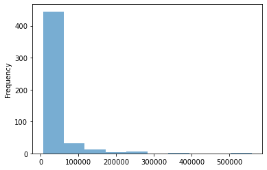
With a DataFrame in hand, we can start working with the data. As an example, below I plot the distribution of revenue among our set of companies. To do so, I first remove the delimiter, and convert the DataFrame column to numeric using pd.to_numeric.
pd.to_numeric(fortune500.revenue.str.replace(',','')).plot.hist(alpha=0.6)
<AxesSubplot:ylabel='Frequency'>

As we can see, the distribution of revenue is strongly right-skewed (positively skewed).
Even though actual applications can of course be more complex, the general principle holds. I hope this simple tutorial was useful.


